93121506 121506 1506 06
The omitted elements on the left side of each argument default to their current values.
If an argument is enclosed in brackets [ ] it is optional and omitting it will cause the command to use a default value which for the time is almost always the current of latest time.
Many commands require you to know a station ID. If you do not know the station ID use the command
stnid name
where name can be any keyword of the location you want. You will also find all the station and buoy IDs in a yellow binder located in the maproom.
When noted, a command may have a `man' (manual) page associated with it. A man page provides additional information about the command. It can be accessed by typing
man command
Also, by appending "-h" to a command a "help screen" will often appear.
td stn same as above but in decoded format for easier reading.
tdd stn shortcut command for abtaining a decoded time series for the past 18 hours.
nw [yymmddhh] lists decoded station observations grouped by to geographic sub-regions in WA, OR, and southwest BC. Only the minimum amount of date/time information need be given. (For example, if you want 21 UTC observations, type "21" in the time field and the most recent 21 UTC observations are displayed.)
pirep stn [ddhh] pilot reports from airport stn for a six hour period beginning with the requested day and hour.
You can also get the most recent aviation observation by typing only the three letter station ID of the following stations:
ast Astoria, OR
bfi Seattle, WA (Boeing Field)
bli Bellingham, WA
eat Wenatchee, WA
geg Spokane, WA
hms Hanford, WA
hqm Hoquiam, WA
nuw Whidbey Island NAS, WA
olm Olympia, WA
pae Everett, WA (Paine Field)
pdx Portland, OR
sea Seattle, WA (Seattle-Tacoma Int'l AP)
smp Stampede Pass, WA
uil Quillayute, WA
ykm Yakima, WA
The command will display nothing if the report is not available.
wacst most recent coastal observations from the Puget Sound area.
tcu stn time series for Coast Guard stations in the United States.
tcc stn time series for coastal observing stations in Canada.
tb stn hourly time series for any fixed buoy location.
tcm stn time series for any Coastal-Marine Automated Network (CMAN) station.
hiway the most recent Cascade Mountains pass reports.
th [stn] time series of hydrometeorological reports from any station in the Cascades and Olympics. If the argument is omitted then a listing of all stations is produced. A listing of hydromet. station names is also in the maproom notebook.
hydro [dd] daily hydrometeorological reports from in the Cascades and Olympics (reports are SHEF encoded). A listing of station names is in the maproom notebook.
snotel stn gives the hourly reports from automatic stations in the mountians. These observations include water equivalent of the snowpack (PILLOW) and the total amount of precipitation that has fallen since the start of the water year (oct. 1). To get a listing of available stations, type snotel -l.
tecol stn gives the time series of observations at Dept. of Ecology stations. Type "tecol -h" for station list.
uwmin [dd] one-minute time series from sensors on the Atmospheric Sciences rooftop. To search for a specific time, at the `more' prompt, type "/hhmm" with a <return> to move to the data beginning at that time (GMT).
uwtail [#min] gives the last #min minutes of rooftop observations in one-minute increments. The default is 30 minutes.
uwhr [dd] hourly time series and 24 hour summaries. The summaries are given at 00 and 12 GMT. The format of the output is as follows:
Hr, # of 1-minute Samples, Pmin, Pmax, Pmean, Tmin, Tmax, Tmean, Wdir, Wsp, Wgst, Precip, Solrad
pdgorge [dd] display the pressure differences between various sites located along the Columbia river gorge for the specified day.
natsum summary of weather conditions across the nation.
wasum summary of weather conditions across Washington.
watab max/min/precip table for Washington stations.
aktab max/min/precip table for Alaska stations.
bctab max/min/precip table for British Columbia stations.
ortab max/min/precip table for Oregon stations.
rnotab max/min/precip table for Nevada stations.
sfotab max/min/precip table for No. California stations.
laxtab max/min/precip table for So. California stations.
phxtab max/min/precip table for Arizona stations.
wazone most recent zone forecasts for the state of Washington.
wast most recent "state" forecasts for the state of Washington.
waxtnd most recent extended range forecasts for the state of Washington.
wadisc most recent technical discussion giving the reasoning behind the forecasts issued by the Seattle WSFO.
wafp4 or watp most recent max/min/pop for selected cities across Washington. Also obtained by typing "fd sea tp".
wamar most recent marine forecasts for Washington.
rainier most recent Mt. Rainier forecast.
The following two commands give forecasts from any forecast office in the United States and Canada. Further information on the forecast offices and regions of coverage may be obtained by typing "man fd".
fd stn [ttt][dd] the "forecast daily" command gives all the forecasts issued over a 24 hour period. The most recent forecast is listed first.
ttt is the type of forecast desired and may be any one of the following:
etaf stn [yymmddhh] same as ngmf but for the ETA model.
ngmv stn [yymmddhh] gives the 12, 24, 36, and 48 hour NGM forecasts which are valid at the time specified by yymmddhh. The last line (TT=0) is the verification for the given day and time. This command is useful for comparing how the NGM model forecasts have evolved over the 48 hour period leading up to the verification time (yymmddhh).
etav stn [yymmddhh] same as ngmv but for ETA model.
The above commands produce output using the following abbreviations:
- A negative temperature or LI is indicated by values greater than 50. To get the actual value, subtract 100 from the coded value. (Ex: A coded value of 97 would mean a true value of -3 (97-100 = -3).
- The yellow binder in the maproom defines more specifically what sigma levels "low, middle, and upper" refer to.
mmos [stn] [dd] MRF MOS city forecast guidance out to eight days.
amos [stn] [ddhh] Aviation MOS guidance for the given city.
If stn is not specified for the above three MOS commands, Seattle (sea) is selected by default.
A command to plot surface observations on a map which allows the user to choose the observation parameters, locations of the map, and the time of the plot. For example, to plot a surface map centered on Wenatchee at 18Z today type "map EAT 18". Type "map -h" for more detailed information.
loopmap loop of the maps of surface obs. over western Washington for the past 9 hours. (See section 7.5 for further information on loop control.)
wxplot [-r] plots a map of station surface data over a specified region and time. The -r "research mode" option allows the user to customize the plot and make hardcopies.
mpps [yymmddhh] shows plotted surface map of Puget Sound region. If ddhh is omitted, the most recent time of observation is drawn.
mpwa [yymmddhh] shows plotted surface map of state of Washington.
mppnw [yymmddhh] shows plotted surface map of Pacific Northwest region.
By appending a "_prt" to the previous three commands, output is also sent to your laser printer. (Ex. "mpwa_prt 2112" prints a map of surface observations in Washington at 12 GMT on the 21st of the current month.)
sond stn [yymmddhh] displays a sounding on a pseudo-adiabatic chart.
skewt stn [yymmddhh] displays a sounding on a skew-T chart.
The next two commands plot two soundings on the same chart. One can either plot soundings of the same station at different times or different stations at the same time. The first station is plotted in black, the second in red. All arguments must be provided.
msond stn1 yymmddhh1 stn2 yymmddhh2
mskewt stn1 yymmddhh1 stn2 yymmddhh2
By appending a "_prt" to these four commands, output is also sent to your laser printer. Ex. "msond_prt uil 92122500 uil 92122512" will overlay the 00 and 12 GMT soundings at Quillayute on 25 Dec 1992 and send the output to the printer.
avis [-t yymmddhh][-l lll][-v vvv][-f ff][-q][-s][-x xdumpfile][outputfile]
plots an isentropic analysis of the most current aviation grid. Variables you can plot are: geopotential height, temperature, U and V wind components, windspeed, Montgomery streamfunction, static stability, pressure, absolute vorticity, and potential vorticity. The default (no arguments) is a plot of potential vorticity of the most recent model run. This program has numerous options which are explained on its `man' page.
ngmis [-t yymmddhh][-l lll][-v vvv][-f ff][-q][-s][-x xdumpfile][outputfile]
same as avis but using NGM data. The options are the same as described on the avis `man' page.
ngmtv [-f ff][-t yymmddhh]
This command creates a plot of 1000-850 mb mean temperature and winds from the NGM initialized on the given date.
-f ff specifies the forecast hour whose value is 0, 12, 24, 36, or 48.
-t yymmddhh gives the initialization date and time and must include year, month, day, and hour.
loopngmtv views a loop of 1000-850 mb mean temperature and winds from the most recent NGM run. The loop cycles through 0 to 48 hour forecasts. (For controlling loops see Section 7.5 "Loop Control" on page15.)
traj The trajectory program allows you to create forward and backward trajectories from NGM-analyzed velocity fields. See the `man' page for specific details in using this program.
ngmsx [ cxstns][gfunc][time][yaxis]
The default command (no arguments) creates a spatial cross-section based on the NGM gridded data at the most recent model initial time from a point over the Pacific Ocean (48,-155) to Wenatchee. Geostrophic wind vectors, relative humidity, and temperatures are plotted.
ngmtx [cxstns][gfunc][time][yaxis]
The default command produces a time cross-section analysis for SEA from the most recent NGM 0 to 48 hour forecast. Geostrophic wind vectors, relative humidity, and temperatures are plotted.
ltnw gives a map of lightning strikes for the Pacific Northwest. User will be prompted for the time and date.
map.lightning yymmdd hh gives a map of lightning strikes for the U.S.
plotspt [yymmddhh] [time_interval] This command plots the soundings from the profiler, where yymmddhh is the ending time and time_interval is the number of hours between each sounding. Defaults are the latest hour for yymmddhh and 1 hour for time_interval. To remove the plot hit return in the plot window.
Note: The following two commands require that the user be configured to use the GEMPAK software.
sp2c [yymmddhh] [NHRS] gives you a graphical display for the lowest 2 kilometers of time-height cross section of data from the profiler, NHRS is the number of hours contained in the cross section. This number must be larger than 3 in order for the command to work. The default setting is 24 hours of data ending at the current time. To quit type gpend in another window.
sp4c [yymmddhh] [NHRS] same as previous command, but the time-height cross-section of the lowest 4 kilometers.
spwt [yymmddhh] gives both the winds and temperatures at various heights for a 12 hour period ending at the time specified. The default ending time is the most recent hour.
spw [yymmddhh] gives only the winds at the same heights as the previous command for 12 hours ending at the specified time.
spt [yymmddhh] same as previous command but for virtual temperature.
tsp -l gives a listing of heights above sea level to choose from when using the command tsp.
tsp ht gives a time series of winds or virtual temperature at the height specified by ht. User will be prompted for beginning and ending times of time series.
tspt gives a time series of virtual temperatures for all heights. User will be prompted for beginning and ending times of time series.
bref [yymmddhh:mm] [elevation_index]
Displays the base reflectivity at one of four elevation angles: 0.5, 1.5, 2.5, and 3.5 degrees (these correspond to elevation_index argument values of 1 to 4).
vel [yymmddhh:mm] [elevation_index]
Displays the field of radial velocity. Elevation angles are specified the same way as for the command bref.
lref [yymmddhh:mm] [elevation_index]
Displays layer maximum reflectivity at one of three vertical layers: 0-24, 24-33, and 33-60 kft (these correspond to elevation_index argument values of 1 to 3)
cref [yymmddhh:mm] Displays composite reflectivity averaged in the vertical.
tops [yymmddhh:mm] Displays echo top heights.
vil [yymmddhh:mm] Displays vertically intergrated liquid water.
pre1 [yymmddhh:mm] Displays one hour precipitation ending at selected time.
pre3 [yymmddhh:mm] Displays three hour precipitation ending at selected time.
pret [yymmddhh:mm] Displays storm total precipitation accumulated up to the selected time.
radar_root [elevation_index] Displays the most recent base reflectivity field on the root window of your X window display. The root window is updated every 3 minutes provided a new image is available. The default value is the same for all commands with an argument of elevation index of 1 (0.5 deg).
The next set of commands allow the user to loop through a time series of radar images. These commands are analogous to the display commands above except they begin with the letter "l" which indicates they loop through a sequence of images determined by the time_specification argument. The time specification takes the form:
[yymmddhh:mm/time_length/time_step]
where yymmddhh:mm is the ending time for the loop which defaults to the current time if not specified. Time_length is the duration of the loop in hours while time_step is the interval of time in hours between images comprising the loop. If not specified time_length defaults to 2 hours while time_step defaults to 0.1 hr, which assures that all available images will be included in the loop.
lbref [time_specification] [elevation_index]
lvel [time_specification] [elevation_index]
llref [time_specification] [elevation_index]
lcref [time_specification]
lpre1 [time_specification]
lpre3 [time_specification]
lpret [time_specification]
ltops [time_specification]
lvil [time_specification]
4.2.1 XAnim -Keyboard Commands
Once the animation is running there are various commands that can be entered into that animation window from the keyboard
Once the animation is running the mouse buttons have the following functions.
<Left_Button> Single step back one frame.
<Middle_Button> Toggle. starts/stops animation.
<Right_Button> Single step forward one frame.
mcidas McIDAS is a program which allows the user to display and loop both visible and infrared satellite imagery, as well as surface, upper air, and gridded data. (See Section 7.0 of this manuel for more information on using McIDAS.) Running this program requires that your account is properly configured.
js Js or Jetstream can display gridded data, surface data, or satellite imagery, launch trajectories, and create loops. This program is flexible enough to allow the user to customize each plot. This program runs under a graphical `windows' interface. See separate `man' page.
avplot Avplot is a menu driven program that allows the user to make custom plots of many different parameters. Similar to Jetstream but not in x-windows format.
wxp This menu driven program can make calculations of meteorological values, analyze and display data, and contour various types of data and variables. This command requires that the UDRESPATH environment variable be properly set. See Ernie Recker or Harry Edmon for more information.
gempak Gempak is a graphical package for displaying various types of parameters. Contact Harry Edman or David Warren for more information and to have your account properly configured.
satir [yymmddhh] View hourly United States infrared images from the GOES 7 satellite.If time is not specified, the most recent available image is shown.
satvis [yymmddhh] same as above but for hourly visible imagery.
satwv [yymmddhh] same as above except for water vapor imagery
1km [yymmddhh] Visible satellite image of Washington state at 1 kilometer resolution. Format of time argument follows yymmddhh:mm. If time is not specified the most recent image is shown. Available at half-hour intervals during daylight hours.
satvisir [yymmddhh] This command loops between the visible and infrared image at the specified time. If time is not specified the most recent images will be shown.
gms.i [yymmddhh] View GMS infrared imagery at specified time. If time is not specified the latest image at 00Z or 12Z is shown.
gms.v [yymmddhh] same as above but for visible imager
eur.i View latest METEOSAT infrared image of Europe.
eur.v same as above but for visible imagery.
uk.i View latest infrared imagery of British Isles.
uk.v same as above but for visible imagery.
meteow.i View latest Atlantic, North and South American full disk images from the METEOSAT backup satellite. If time is not specified the latest image at 00Z or 12Z is shown.
meteow.v same as above but for visible imagery.
meteoe.i View latest full disk images of Europe and Africa from the METEOSAT satellite.
meteoe.v same as above but for visible imagery.
These next commands loop the U.S. and Washington state satellite images. The time specification takes the form:
[yymmddhh:mm/time_length/time_step]
where yymmddhh is the ending time for the loop which defaults to the current time if not specified. Time_length is the duration of the loop in hours while time_step is the interval of time in hours between images comprising the loop. If not specified time_length defaults to 2 hours while time_step defaults to 1 hr which assures that all available images will be included in the loop.
lir [time_spec] Loops the U.S. infrared images.
lvis [time_spec] Loops the U.S. visible images.
l1km [time_spec] Loops the Washington state 1 kilometer visible images.
McIDAS is far too complex to describe in detail here. Only a few simple commands are included to get you going. A more detailed description of all commands is located in a blue binder in the maproom.
DF aatt frame# EC xxx [mag]
This command will display a satellite image in the image window..
Currently, we retain only the last 24 hours of McIDAS images. To see which ones are available type
LA aatt1 aatt2 lists areas between areas aatt1 and aatt2. Output is in the blue text window.
Once you plot an IR or visible satellite image, you must enter a separate command to draw a map on the image. First, make sure the image window is displaying the correct frame then type:
MAP [H] draws a map in the image window. The optional `H' will cause state boundaries to be drawn.
BATCH [arguments] "program name
executes batch program called program name. Arguments may or may not be required, depending on the specific batch program.
As of this date, the following are acceptable BATCH program names:
tt xxx "IRZOOM , or
tt xxx "VSZOOM
Creates a loop of four images at time tt centered on station xxx with consecutively increasing magnification.
"IR500 draws the latest 12 GMT IR image and overlays the 500mb countours.
For example, to create a loop of visible images zooming onto Seattle at 18 GMT enter, BATCH 18 SEA "VSZOOM
Figure 2 is the local weather data and forecasts page.
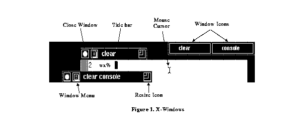
open window Put cursor in a window icon at top of screen and press left mouse button.
close window Put cursor in a window icon or circle at left of title bar and press left mouse button.
move window Put cursor in shaded area in title bar of window, hold the middle mouse button, and drag to new location.
resize window Put cursor in resize icon at right of title bar, hold the middle mouse button, drag mouse to window border, and resize window to desired size.
bring to front
(raise) window Put cursor on title bar and press left mouse button. If the title bar is hidden, put cursor in window icon and press middle mouse button.
send to back
(lower) window Put cursor on title bar and press right mouse button.
kill window Put cursor in menu icon in title bar, hold the middle mouse button, drag mouse to select `kill', and release mouse button.
Some of the above commands may also be performed by pointing the cursor in a region without any windows, holding down the middle mouse button, and selecting the desired action, then you have to go back to the window you want the action preformed in.
- Local surface station plots
- Local soundings
- Loops
- Jetstream
- Forecast map
- Surface analysis/radar summary
- Recent visible satellite image
- Recent IR satellite image
Point the cursor in empty space, hold the right mouse button, and drag to your selection. If there is a menu icon at the right of the selection bar, drag the mouse to the right for more choices. Note that for many programs it takes several seconds or longer for any display or effect to occur.
middle Toggles loop mode on/off. When holding the <shift> key down and pressing this button, the loop is killed and you are returned to the prompt.
right When loop mode is off, pressing this button advances one frame in the loop sequence.
When loop mode is on, this button increases the loop speed. Holding the <shift> key down and pressing the right button will decrease the pause at the end of the loop.
left When loop mode is off, pressing this button moves back one frame.
When loop mode is on, this button decreases the loop speed. Holding the <shift> key down and pressing the left button will increase the pause at the end of the loop.