Beginning with GMT version 2.1.4, ``Example 11'' was included in the cookbook. The example makes an RGB color cube by a simple awk script. We wrote a program to compute HSV grids for each face of this cube, and include a version of the cube with HSV contours on it as file contoured_cube.ps in /share.
In this appendix, we are going to try to explain the relationship between the RGB and HSV color systems so as to (hopefully) make them more intuitive. GMT allows users to specify colors in cpt files in either system (colors on command lines, such as pen colors in -W option, are always in RGB). GMT uses the HSV system to achieve artificial illumination of colored images (e.g. -I option in grdimage) by changing the s and v coordinates of the color. When the intensity is zero, the data are colored according to the cpt file. If the intensity is non-zero, the data are given a starting color from the cptfile but this color (after conversion to HSV if necessary) is then changed by moving (s,v) toward HSV_MIN_SATURATION, HSV_MIN_VALUE if the intensity is negative, or toward HSV_MAX_SATURATION, HSV_MAX_VALUE if positive. These are defined in the .gmtdefaults4 file and are usually chosen so the corresponding points are nearly black (s = 1, v = 0) and white (s = 0, v = 1). The reason this works is that the HSV system allows movements in color space which correspond more closely to what we mean by ``tint'' and ``shade''; an instruction like ``add white'' is easy in HSV and not so obvious in RGB.
We are going to try to give you a geometric picture of color
mixing in HSV from a tour of the RGB cube. The geometric
picture is helpful, we think, since HSV are not orthogonal
coordinates and not found from RGB by an algebraic transformation.
But before we begin traveling on the RGB cube, let us give two
formulae, since an equation is often worth a thousand words.
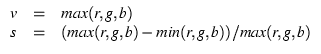
Note that when ![]() (black), the expression for s
gives 0/0; black is a singular point for s. The expression
for h is not easily given without lots of ``if'' tests, but
has a simple geometric explanation. So here goes: Look at the
cube face with black, red, magenta, and blue corners.
This is the g = 0 face. Orient the cube so that you are
looking at this face with black in the lower left corner. Now
imagine a right-handed cartesian (r, g, b) coordinate system
with origin at the black point; you are looking at the
(black), the expression for s
gives 0/0; black is a singular point for s. The expression
for h is not easily given without lots of ``if'' tests, but
has a simple geometric explanation. So here goes: Look at the
cube face with black, red, magenta, and blue corners.
This is the g = 0 face. Orient the cube so that you are
looking at this face with black in the lower left corner. Now
imagine a right-handed cartesian (r, g, b) coordinate system
with origin at the black point; you are looking at the ![]() plane with r increasing to your right, g increasing
away from you, and b increasing up. Keep this sense of
(r, g, b) as you look at the cube.
plane with r increasing to your right, g increasing
away from you, and b increasing up. Keep this sense of
(r, g, b) as you look at the cube.
The RGB color cube has six faces. On three of these one of
(r, g, b) is equal to 0. These three faces meet at the
black corner, where ![]() . On these three faces
saturation, the S in HSV, has its maximum value; s = 1
on these faces. (Accept this definition and ignore the s
singularity at black for now). Therefore h and v are
contoured on these faces; h in gray solid lines and v
in white dashed lines (v ranges from 0 to 1 and is contoured
in steps of 0.1).
. On these three faces
saturation, the S in HSV, has its maximum value; s = 1
on these faces. (Accept this definition and ignore the s
singularity at black for now). Therefore h and v are
contoured on these faces; h in gray solid lines and v
in white dashed lines (v ranges from 0 to 1 and is contoured
in steps of 0.1).
On the other three faces one of (r, g, b) is equal to the
maximum value. These three faces meet at the white corner, where
![]() . On these three faces value, the V in HSV, has
its maximum value; v = 1 on these faces. Therefore h
and s are contoured on these faces; h in gray solid
lines and s in black dashed lines (s ranges from 0 to
1 with contours every 0.1).
. On these three faces value, the V in HSV, has
its maximum value; v = 1 on these faces. Therefore h
and s are contoured on these faces; h in gray solid
lines and s in black dashed lines (s ranges from 0 to
1 with contours every 0.1).
The three faces where v = 1 meet the three faces where ![]() in six edges where both
in six edges where both ![]() (and at least one of (r, g, b)
= 0 and at least one of (r, g, b) = 255). Trace your finger
around these edges, starting at the red point and moving to the yellow
point, then on around. You will visit six of the eight corners of the
cube, in this order: red (
(and at least one of (r, g, b)
= 0 and at least one of (r, g, b) = 255). Trace your finger
around these edges, starting at the red point and moving to the yellow
point, then on around. You will visit six of the eight corners of the
cube, in this order: red (![]() ); yellow (
); yellow (![]() ); green
(
); green
(![]() ); cyan (
); cyan (![]() ); blue (
); blue (![]() ); magenta
(
); magenta
(![]() ). Three of these are the RGB colors; the other three
are the CMY colors which are the complement of RGB and are used in many
color hardcopy devices (color monitors usually use RGB). The only cube
corners you did not visit on this path are the black and white corners.
Imagine an axis running through the black and white corners. If you
project the RYGCBM edge path onto a plane perpendicular to the black-white
axis, the path will look like a hexagon, with RYGCBM at the vertices,
every 60
). Three of these are the RGB colors; the other three
are the CMY colors which are the complement of RGB and are used in many
color hardcopy devices (color monitors usually use RGB). The only cube
corners you did not visit on this path are the black and white corners.
Imagine an axis running through the black and white corners. If you
project the RYGCBM edge path onto a plane perpendicular to the black-white
axis, the path will look like a hexagon, with RYGCBM at the vertices,
every 60![]() apart. Now we can make a geometric definition of hue:
Take a vector from the origin (black point) to any point in the cube;
project this vector onto the plane with the RYGCBM hexagon; then hue is
the angle this projected vector makes with the R direction on the hexagon.
Thus hue is an angle describing rotation around the black-white axis.
Note that by this definition, if a point is on the black-white axis, its
(r, g, b) vector will project as a point at the center of the
hexagon, so its hue is undefined. Points on the black-white axis have
apart. Now we can make a geometric definition of hue:
Take a vector from the origin (black point) to any point in the cube;
project this vector onto the plane with the RYGCBM hexagon; then hue is
the angle this projected vector makes with the R direction on the hexagon.
Thus hue is an angle describing rotation around the black-white axis.
Note that by this definition, if a point is on the black-white axis, its
(r, g, b) vector will project as a point at the center of the
hexagon, so its hue is undefined. Points on the black-white axis have
![]() , and they are shades of gray; we will call the black-white
axis the gray axis.
, and they are shades of gray; we will call the black-white
axis the gray axis.
Let us call the points where ![]() (the points on the RYGCBM
path of cube edges) the ``pure'' colors. If we start at a pure color
and we want to whiten it, we can keep h constant and
(the points on the RYGCBM
path of cube edges) the ``pure'' colors. If we start at a pure color
and we want to whiten it, we can keep h constant and ![]() while decreasing s; this will move us along one of the cube
faces toward the white point. If we start at a pure color and we want
to blacken it, we can keep h constant and
while decreasing s; this will move us along one of the cube
faces toward the white point. If we start at a pure color and we want
to blacken it, we can keep h constant and ![]() while decreasing
v; this will move us along one of the cube faces toward the black
point. Any point in (r, g, b) space which can be thought of as a
mixture of pure color + white, or pure color + black, is on a face of
the cube.
while decreasing
v; this will move us along one of the cube faces toward the black
point. Any point in (r, g, b) space which can be thought of as a
mixture of pure color + white, or pure color + black, is on a face of
the cube.
The points in the interior of the cube are a little harder to describe.
The definition for h above works at all points in (non-gray)
(r, g, b) space, but so far we have only looked at (s,
v) on the cube faces, not inside it. At interior points, none
of (r, g, b) is equal to either 0 or 255. Choose such a point,
not on the gray axis. Now draw a line through your point so that the
line intersects the gray axis and also intersects the RYGCBM path of
edges somewhere. It is always possible to construct this line, and
all points on this line have the same hue. This construction shows
that any point in RGB space can be thought of as a mixture of a pure
color plus a shade of gray. If we move along this line away from the
gray axis toward the pure color, we are ``purifying'' the color by
``removing gray''; this move increases the color's saturation. When
we get to the point where we cannot remove any more gray, at least one
of (r, g, b) will have become zero and the color is now fully
saturated; ![]() . Conversely, any point on the gray axis is
completely undersaturated, so that
. Conversely, any point on the gray axis is
completely undersaturated, so that ![]() there. Now we see that
the black point is special, because it is the intersection of three
planes on which
there. Now we see that
the black point is special, because it is the intersection of three
planes on which ![]() , but it is on a line where
, but it is on a line where ![]() ; it is a
singular point, and we get ``0/0'' in the above formula. We see also
that saturation is a measure of ``purity'' or ``vividness'' of the
color.
; it is a
singular point, and we get ``0/0'' in the above formula. We see also
that saturation is a measure of ``purity'' or ``vividness'' of the
color.
It remains to define value, and the formula above is really the best
definition. But if you like our geometric constructions, try this:
Take your point in RGB space and construct a line through it so that
this line goes through the black point; produce this line from black
past your point until it hits a face on which ![]() . All points
on this line have the same hue. Note that this line and the line we
made in the previous paragraph are both contained in the plane whose
equation is hue = constant. These two lines meet at some arbitrary
angle which varies depending on which point you chose. Thus HSV is
not an orthogonal coordinate system. If the line you made in the
previous paragraph happened to touch the gray axis at the black point,
then these two lines are the same line, which is why the black point
is special. Now, the line we made in this paragraph illustrates the
following: If your chosen point is not already at the end of the
line, where
. All points
on this line have the same hue. Note that this line and the line we
made in the previous paragraph are both contained in the plane whose
equation is hue = constant. These two lines meet at some arbitrary
angle which varies depending on which point you chose. Thus HSV is
not an orthogonal coordinate system. If the line you made in the
previous paragraph happened to touch the gray axis at the black point,
then these two lines are the same line, which is why the black point
is special. Now, the line we made in this paragraph illustrates the
following: If your chosen point is not already at the end of the
line, where ![]() , then it is possible to move along the line in
that direction so as to increase (r, g, b) while keeping the
same hue. The effect this has on a color monitor is to make the
color shine more brightly, but ``brightness'' has other meanings in
color geometry, so let us say that if you can move in this way, you
can make your hue ``stronger''; if you are already on a plane where
at least one of (r, g, b) = 255, then you cannot get a stronger
version of the same hue. Thus, v measures strength. Note that
it is not quite true to say that v measures distance away from
the black point, because v is not equal to
, then it is possible to move along the line in
that direction so as to increase (r, g, b) while keeping the
same hue. The effect this has on a color monitor is to make the
color shine more brightly, but ``brightness'' has other meanings in
color geometry, so let us say that if you can move in this way, you
can make your hue ``stronger''; if you are already on a plane where
at least one of (r, g, b) = 255, then you cannot get a stronger
version of the same hue. Thus, v measures strength. Note that
it is not quite true to say that v measures distance away from
the black point, because v is not equal to
![]() .
.
The RGB system is understandable because it is cartesian, and we all learned cartesian coordinates in school. But it doesn't help us create a tint or shade of a color; we cannot say, ``We want orange, and a lighter shade of orange, or a less vivid orange''. With HSV we can do this, by saying, ``Orange must be between red and yellow, so its hue is about h = 30; a less vivid orange has a lesser s, a darker orange has a lesser v''. On the other hand, the HSV system is a peculiar geometric construction, it is not an orthogonal coordinate system, and it is not found by a matrix transformation of RGB; these make it difficult in some cases too. Note that a move toward black or a move toward white will change both s and v, in the general case of an interior point in the cube. The HSV system also doesn't behave well for very dark colors, where the gray point is near black and the two lines we constructed above are almost parallel. If you are trying to create nice colors for drawing chocolates, for example, you may be better off guessing in RGB coordinates.
Well, there you have it, folks. We've been doing GMT for 10 years and all we know about color can be written in about 2 pages. We hope we haven't told you any lies. For more details, you should consult a book about color systems. But as example 11 shows, a lot can be learned by experimenting with GMT tools. Our thanks to John Lillibridge for Example 11.