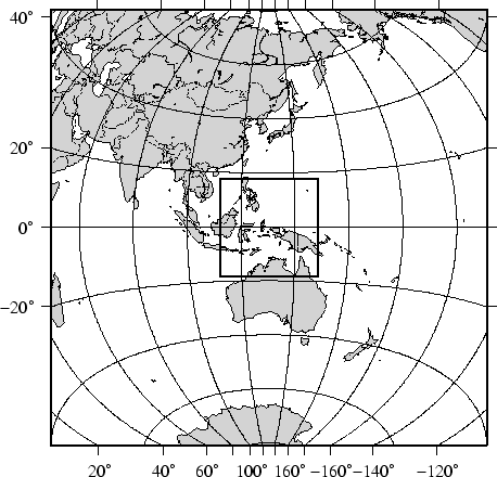
We begin with an azimuthal equidistant map of the hemisphere
centered on 130![]() 21'E, 0
21'E, 0![]() 12'S, which is slightly west
of New Guinea, near the Strait of Dampier. The edges of the
map are all 9000 km true distance from the projection center.
At this scale (and for global maps) the crude resolution data
will usually be adequate to capture the main geographic features.
To avoid cluttering the map with insignificant detail we only
plot features (i.e., polygons) that exceed 500 km
12'S, which is slightly west
of New Guinea, near the Strait of Dampier. The edges of the
map are all 9000 km true distance from the projection center.
At this scale (and for global maps) the crude resolution data
will usually be adequate to capture the main geographic features.
To avoid cluttering the map with insignificant detail we only
plot features (i.e., polygons) that exceed 500 km![]() in area.
Smaller features would only occupy a few pixels on the plot and
make the map look ``dirty''. We also add national borders to
the plot. The crude database is heavily decimated and simplified
by the DP-routine: The total file size of the coastlines, rivers,
and borders is only 286 Kbytes. The plot is produced by the
command (the box indicates the outline of the next map):
in area.
Smaller features would only occupy a few pixels on the plot and
make the map look ``dirty''. We also add national borders to
the plot. The crude database is heavily decimated and simplified
by the DP-routine: The total file size of the coastlines, rivers,
and borders is only 286 Kbytes. The plot is produced by the
command (the box indicates the outline of the next map):
gmtset GRID_CROSS_SIZE_PRIMARY 0 OBLIQUE_ANNOTATION 22 ANNOT_MIN_SPACING 0.3
pscoast `./getbox -JE130.35/-0.2/1i -9000 9000 -9000 9000` -JE130.35/-0.2/3.5i -P -Dc \
   -A500 -Glightgray -W0.25p -N1/0.25tap -B20g20WSne -K > GMT_App_K_1.ps
./getrect -JE130.35/-0.2/1i -2000 2000 -2000 2000 | psxy -R -JE130.35/-0.2/3.5i -O -W1.5p -L -A \
   >> GMT_App_K_1.ps
Here, we use the OBLIQUE_ANNOTATION bit flags to achieve horizontal annotations and set ANNOT_MIN_SPACING to suppress some longitudinal annotations near the S pole that otherwise would overprint.