Here is the basemap python code that was used to generate this plot from this WRF output file:
from netCDF4 import Dataset as NetCDFFile
from mpl_toolkits.basemap import Basemap
import matplotlib.pyplot as plt
import numpy as np
import sys
# allow specification of the wrfout file on the command line.
if (len(sys.argv) > 1):
ncfile = sys.argv[1]
else:
ncfile = 'wrfout_d1.uvrewrite.nc'
print 'Using wrfout file: "','\b'+ncfile,'\b"' # use \b to delete space
nc = NetCDFFile(ncfile, 'r')
#
# CEN_LAT and CEN_LON are specific to the nest and are not
# actually what you want. If available, you should use
# MOAD_CEN_LAT and STAND_LON
cenlat = nc.getncattr('CEN_LAT')
cenlon = nc.getncattr('CEN_LON')
cenlon = nc.getncattr('STAND_LON')
cenlat = nc.getncattr('MOAD_CEN_LAT')
lat1 = nc.getncattr('TRUELAT1')
lat2 = nc.getncattr('TRUELAT2')
#
# get the actual longitudes, latitudes, and corners
lons = nc.variables['XLONG'][0]
lats = nc.variables['XLAT'][0]
lllon = lons[0,0]
lllat = lats[0,0]
urlon = lons[-1,-1]
urlat = lats[-1,-1]
#
# get the grid-relative wind components and covert from m/s to knots
ur = nc.variables['U10'][0] * 1.94386
vr = nc.variables['V10'][0] * 1.94386
#
# get the WRF local cosine and sines of the map rotation
cosalpha = nc.variables['COSALPHA'][0]
sinalpha = nc.variables['SINALPHA'][0]
#
# get the temperature field to plot a background color contour
t2m = nc.variables['T2'][0]
#
# Make our map which is on a completely different projection.
# To illustrate the problems, go to the upper right corner of the domain,
# or lower right corner in the southern hemisphere, where the distortion
# is the greatest
fig = plt.figure(1, figsize=(12.92, 9.85))
ax = plt.subplot(111)
if urlat >= 0:
map = Basemap(projection='cyl',llcrnrlat=urlat-5,urcrnrlat=urlat+3,
llcrnrlon=urlon-10,urcrnrlon=urlon,
resolution='h')
else:
map = Basemap(projection='cyl',llcrnrlat=lllat-5,urcrnrlat=lllat+3,
llcrnrlon=lllon,urcrnrlon=lllon+10,
resolution='h')
#
x, y = map(lons[:,:], lats[:,:])
cf = map.contourf(x, y, t2m, alpha = 0.4)
#plt.colorbar(cf, orientation='horizontal', pad=0, aspect=50)
#
# overlay wind barbs doing nothing to show the problem
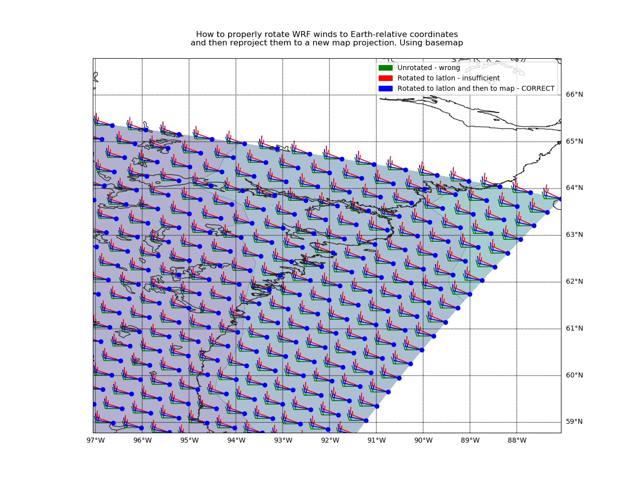
map.barbs(x, y, ur, vr, color='green',label='Unrotated - wrong')
# rotate winds to earth-relative using the correct formulas
ue = ur * cosalpha - vr * sinalpha
ve = vr * cosalpha + ur * sinalpha
# overlay wind barbs using the earth-relative winds showing we're still wrong
map.barbs(x, y, ue, ve, color='red',label='Rotated to latlon - insufficient')
# now rotate our earth-relative winds to the x/y space of this map projection
urot, vrot = map.rotate_vector(ue,ve,lons,lats)
map.barbs(x, y, urot, vrot, color='blue',label='Rotated to latlon and then to map - CORRECT')
# finish up map drawing
parallels = np.arange(-85.,85,1.)
meridians = np.arange(-180.,180.,1.)
map.drawcoastlines(color = '0.15')
map.drawparallels(parallels,labels=[False,True,True,False])
map.drawmeridians(meridians,labels=[True,False,False,True])
# add a legend.
# NOTE: for wind barb/vector plots, each component of the wind got its own
# legend entry, so this line
# plt.legend()
# resulted in duplication. The next 3 lines handle sifting the legend.
#ax = plt.gca()
handles, labels = ax.get_legend_handles_labels()
legend = plt.legend([handles[0],handles[2],handles[4]], [labels[0],labels[2],labels[4]],loc='upper right')
#
# plot the points of the grid to illustrate where the vectors should be pointing
map.plot(x,y,'bo')
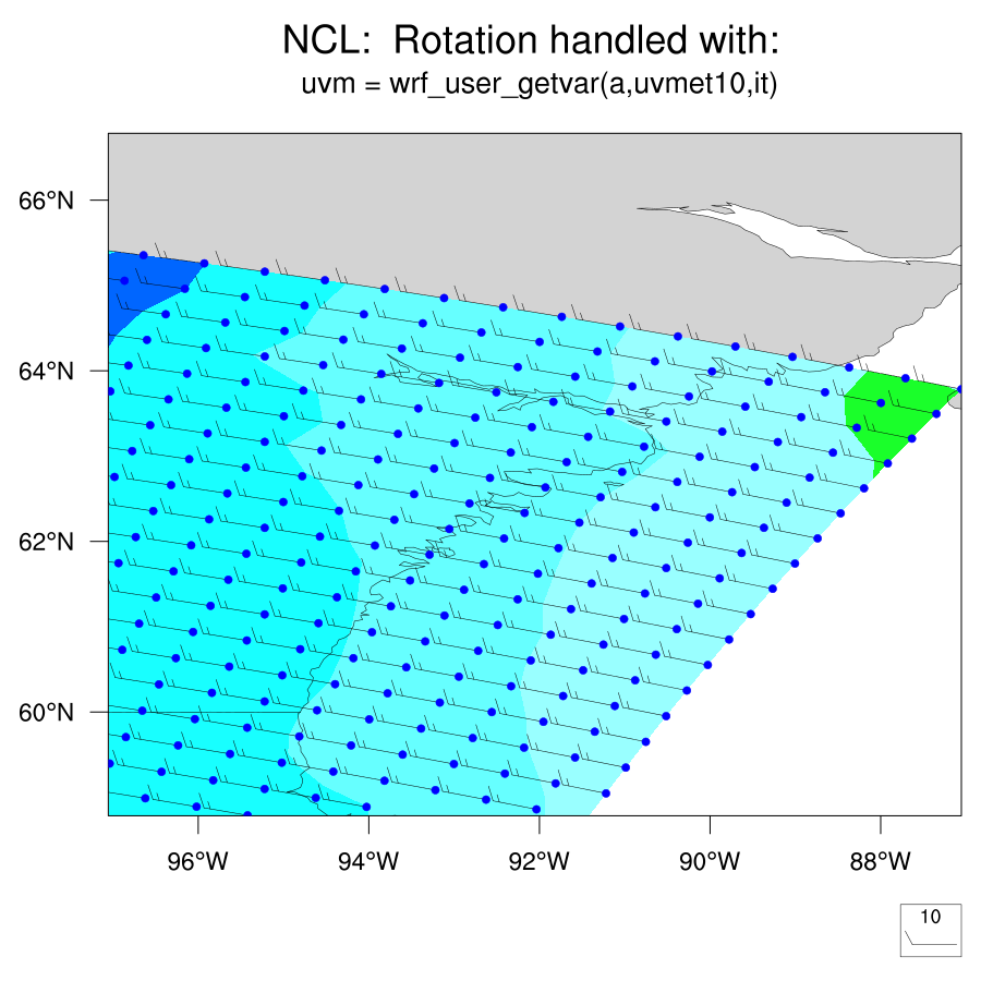
plt.title('How to properly rotate WRF winds to Earth-relative coordinates\nand then reproject them to a new map projection. Using basemap\n')
#plt.show()
plt.savefig('basemapwinds.jpg')
Here is the cartopy python code that was used to generate this plot from this WRF output file:
######################################################################
# Import the needed modules.
#
import cartopy.crs as ccrs
import cartopy.feature as cfeature
import matplotlib.pyplot as plt
import numpy as np
import xarray as xr
from cartopy.mpl.gridliner import LONGITUDE_FORMATTER, LATITUDE_FORMATTER
######################################################################
# The following code reads the example data using the xarray open_dataset
# function and prints the coordinate values that are associated with the
# various variables contained within the file.
ds = xr.open_dataset('wrfout_d1.uvrewrite.nc')
ds.coords
# Grab lat/lon values
lats = ds.XLAT.data[0]
lons = ds.XLONG.data[0]
lllon = lons[0][0]
lllat = lats[0][0]
urlon = lons[-1][-1]
urlat = lats[-1][-1]
# Select and grab data
t2m = ds['T2'].data[0]
uwnd = ds['U10']
vwnd = ds['V10']
cosalpha = ds['COSALPHA']
sinalpha = ds['SINALPHA']
# properly convert to earth-relative U and V and convert m/s to kt
ue = 1.94386 *(uwnd.data[0]*cosalpha.data[0] - vwnd.data[0]*sinalpha.data[0])
ve = 1.94386 *(vwnd.data[0]*cosalpha.data[0] + uwnd.data[0]*sinalpha.data[0])
# make grid-relative U and V in knots
ukt = 1.94386 * uwnd.data[0]
vkt = 1.94386 * vwnd.data[0]
# Set up the projection of the data; if lat/lon then PlateCarree is what you want
plotcrs = ccrs.PlateCarree()
# this correction comes from
# https://github.com/SciTools/cartopy/issues/1179
rho = np.pi/180.
u_src_crs = ue / np.cos(lats*rho)
v_src_crs = ve
magnitude = np.sqrt(ue**2 + ve**2)
magn_src_crs = np.sqrt(u_src_crs**2 + v_src_crs**2)
ux = u_src_crs * magnitude / magn_src_crs
vx = v_src_crs * magnitude / magn_src_crs
# Set up the projection that this WRF model actually uses
#datacrs = ccrs.LambertConformal(central_longitude=-121.0,
# central_latitude=45.66481,
# standard_parallels=(60, 30),
# globe=ccrs.Globe(ellipse='WGS84',semimajor_axis=6370000.,semiminor_axis=6370000.))
# The following
# ux,vx = datacrs.transform_vectors(plotcrs,lons,lats,ue,ve)
# should have worked, but it the U component
# you retrieve needs to be divided by cos(lat) to get the
# direction correct, but then you mess up the magnitude.
# That's why we had to calculate ux and vx on our own above.
##
# Start the figure and create plot axes with proper projection
fig = plt.figure(1, figsize=(12.92, 9.85))
ax = plt.subplot(111, projection=plotcrs)
if urlat >= 0:
ax.set_extent([urlon-10, urlon, urlat-5, urlat+3], plotcrs)
else:
ax.set_extent([lllon, lllon+10, lllat-5, lllat+3], plotcrs)
# Add geopolitical boundaries for map reference
states = cfeature.NaturalEarthFeature(category="cultural", scale="50m",
facecolor="none",
name="admin_1_states_provinces_shp")
ax.add_feature(states, linewidth=0.5, edgecolor="black")
ax.coastlines('50m', linewidth=0.8)
ax.add_feature(cfeature.COASTLINE.with_scale('50m'))
ax.add_feature(cfeature.STATES.with_scale('50m'))
# Plot 500-hPa wind barbs in knots, regrid to reduce number of barbs
# Plot 500-hPa wind barbs in knots, regrid to reduce number of barbs
levs = np.arange(234,288,6)
cf = ax.contourf(lons, lats, t2m, levs, alpha = 0.4, transform=plotcrs)
#plt.colorbar(cf, orientation='horizontal', pad=0, aspect=50)
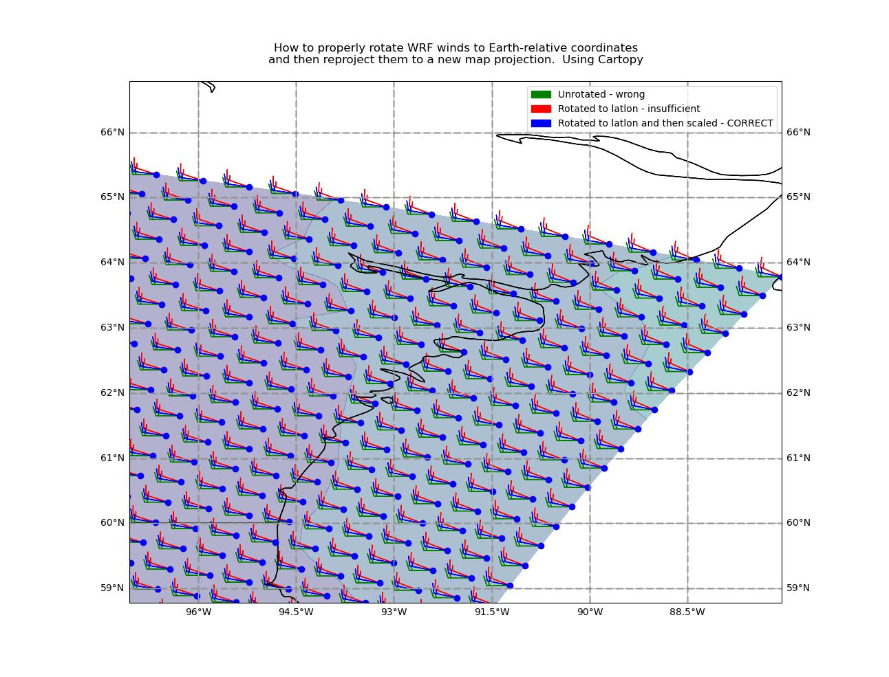
ax.barbs(lons, lats, ukt, vkt, pivot='tip',
color='green', transform=plotcrs,label='Unrotated - wrong')
ax.barbs(lons, lats, ue, ve, pivot='tip',
color='red', transform=plotcrs,label='Rotated to latlon - insufficient')
ax.barbs(lons, lats, ux, vx, pivot='tip',
color='blue', transform=plotcrs,label='Rotated to latlon and then scaled - CORRECT')
# Make some nice titles for the plot (one right, one left)
ax = plt.gca()
handles, labels = ax.get_legend_handles_labels()
legend = plt.legend([handles[0],handles[1],handles[2]], [labels[0],labels[1],labels[2]])
# plot the points of the grid to illustrate where the vectors should be pointing
ax.plot(lons,lats,'bo', transform=plotcrs)
ax.gridlines()
plt.title('How to properly rotate WRF winds to Earth-relative coordinates\nand then reproject them to a new map projection. Using Cartopy\n')
gl = ax.gridlines(crs=ccrs.PlateCarree(), draw_labels=True,
linewidth=2, color='gray', alpha=0.5, linestyle='--')
gl.top_labels = False
gl.xformatter = LONGITUDE_FORMATTER
gl.yformatter = LATITUDE_FORMATTER
gl.ylabel_style = {'size': 10, 'color': 'black'}
gl.xlabel_style = {'size': 10, 'color': 'black'}
plt.savefig('cartopywinds.jpg')